..

Statistics - Sampling and tendency

Often, we learn to use machine learning models without knowing the logic behind them. The intention of this series is to show the basis of these models so that we can apply them in better ways in our work, thereby increasing the quality of knowledge.

Statistical Analysis

Statistics is the science that uses probabilistic theories to explain the frequency of event occurrences. We have some subclasses within statistics, these are:

Descriptive Statistics

Descriptive statistics aim to summarize and describe any set of data. We use it in the exploratory analysis and presentation of data.

Probabilistic Statistics

This aims to analyze phenomena in which the result, even under equal conditions, varies according to experiments. For example, in a dice game, what is the probability of two dice showing a 6 on top?

The answer is 16.6%.

Inferential Statistics

Finally, this is concerned with the analysis and interpretation of these data. For example, calculating the preference votes of voters for a politician. These analyses are made from a fraction (sample) of voters within a whole.

Types of Research

Observation

Analyzes phenomena without any interaction in the environment, meaning the phenomena do not undergo any alteration. Vaccine tests, for example.

Experiment

Different groups are treated differently within N scenarios. Again, we can use the analysis of preference votes as an example.

Variable Types

Numeric Quantitative

It can be defined as Continuous, with real values and can have any interval, for example, the number in a measurement, 12.3 cm. Or Discrete, being immutable integer numbers that can be within a range, for example, the number of people in a village.

Categorical Quantitative

They are divided into Nominal variables, which are categories without hierarchy, an example of this are geometric shapes, as they do not follow any type of ordering. Or Ordinal, which have hierarchy, the best example for this category is army ranks.

Data Analysis

Often when we encounter different types of data (especially if it’s a very large dataset), we become blind to some details and thus fail to synthesize these data for information. And it is so that we do not lose these details that we use exploratory analysis, with it we can obtain variations, anomalies, trends, and patterns of these data. There is a subtle science in exploratory analysis, plotting graphs is not data exploration, but exploring data consequently generates information that can be plotted in graphs.

Sampling

A sample is a random fraction taken (inference) from a group, all individuals in this group must have the same chance of being chosen as a sample. This sample should demonstrate the characteristics of the group from which it was taken.

The main types of sampling

Simple Random Sampling

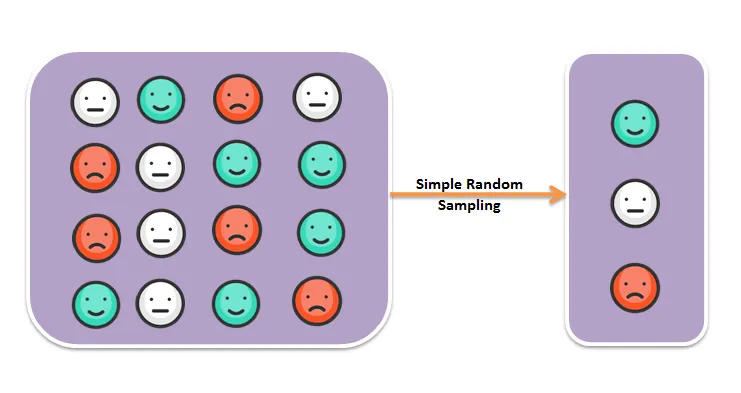
A certain number is randomly drawn from a population group, where all elements of the population have the same chances of being chosen to compose the sample.

Example: We have a group of students in a classroom, and we draw a sample randomly. In the first round of selection, student “A” is drawn.

If there is a possibility of drawing the same student in the following rounds, it’s called Simple Random Sampling with Replacement because we return the student to the group afterward.

If we cannot select student “A” again, it’s called Simple Random Sampling without Replacement, meaning we do not return the student to the group again.

Examples with Iris

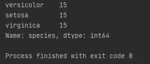
Simple Random Sampling

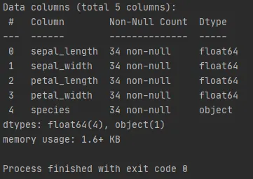
More information about the database

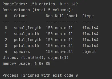
To take a sample from this database, we use the function sample(n = N), where N is the total number of samples to be drawn, and sample.info() to return the generated sample.

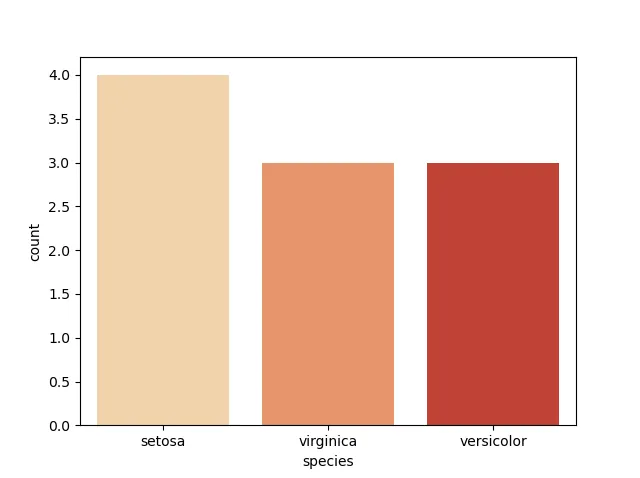
Instead of using integer numbers, it’s possible to take a sample based on the percentage of the population using sample(frac = 0.N), where N is the fractional size of the sample.

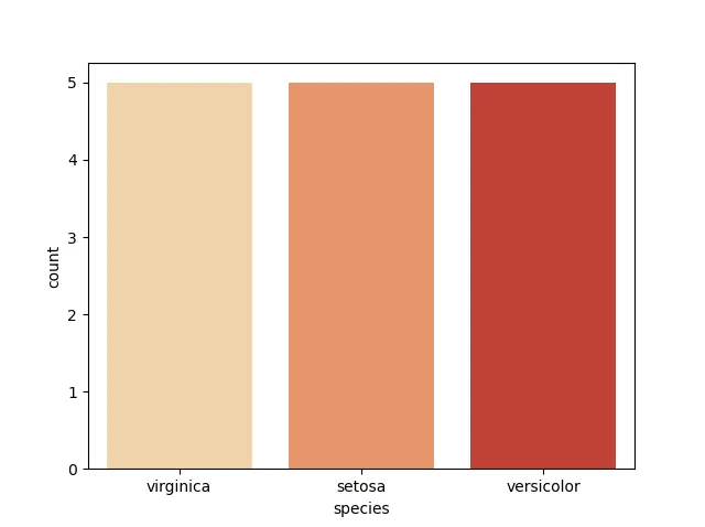
Stratified Random Sampling

This sampling method divides the entire population into strata (groups), ensuring that no individual is left out and that each individual belongs to only one group.

For example, if we need to choose 200 students from 4 different colleges, we would require 4 random samples, each with 50 students.

We can use Scikit-Learn for this type of sampling.

To generate the sample:

We use stratify=Attribute[’N’] to generate the sample.

Test_size=N indicates the amount of data we want in a sample. In the example below, test_size=0.30 would be equal to 30% of the total quantity of the specified attribute.

We use y_test.shape to return the number of records in the test set. This set will be divided to form the groups.

The variables train and test work as follows: all variables in train are used precisely to train the model with the provided data, while the variables in test use data unseen by the training models. This way, we have metrics on how the model handles this data.

For a better understanding of the train_test_split method, I suggest reading this answer: How does the train_test_split method work in scikit-learn?

Systematic Sampling

It is based on first randomly selecting an individual from the population. After that, every Nth individual, relative to the sampling unit (the first individual selected from the population), is chosen for the sample. For example, in a list of names, we would select one name every 10 names.

Attention: If the samples are not selected randomly, they will become biased and invalid for research purposes.

Measures of Central Tendency

These measures represent the data in a more condensed form than in a table, being a calculated value whose result represents the population.

Within these measures, we have:

Arithmetic Mean

The mean is the sum of all values divided by the number of items summed. For example, calculating the average salary of a group of employees.

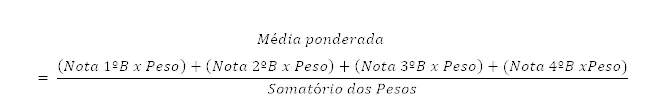
Weighted Mean

The weighted mean is calculated by multiplying each value in the set by its weight, then dividing this result by the sum of the weights.

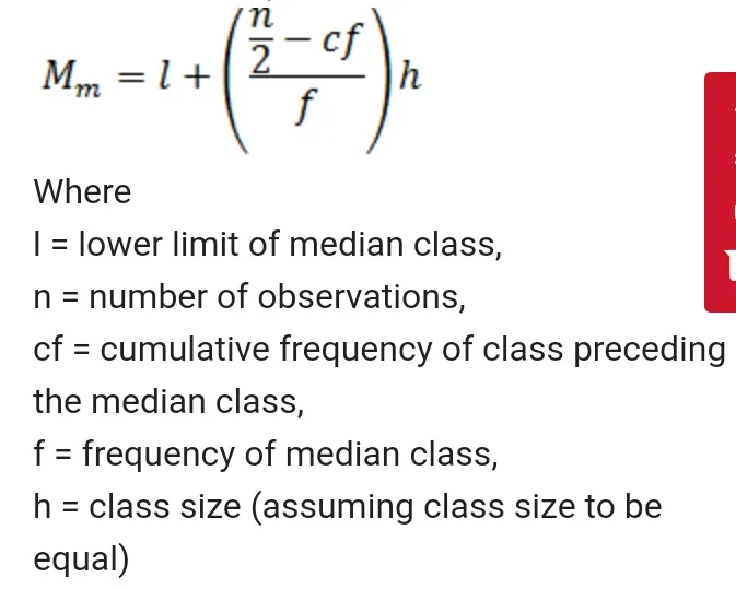
Median

The median is the central value in a sequence of values. If there are two central values, the median is the average of these two values.

Mode

Mode is a measure of central tendency. It returns the most frequently occurring data in a group and can also be used with non-numeric resources.

Thanks, bye!

References

All credits to the original sources for the images used in this document.